Volume 14, No. 3, Art. 15 – September 2013
An Introduction to Applied Data Analysis with Qualitative Comparative Analysis (QCA)
Nicolas Legewie
Abstract: The key to using an analytic method is to understand its underlying logic and figure out how to incorporate it into the research process. In the case of Qualitative Comparative Analysis (QCA), so far these issues have been addressed only partly. While general introductions and user's guides for QCA software packages are available, prospective users find little guidance as to how the method works in applied data analysis. How can QCA be used to produce comprehensive, ingenious explanations of social phenomena?
In this article, I provide such a hands-on introduction to QCA. In the first two parts, I offer a concise overview of 1. the method's main principles and advantages as well as 2. its vital concepts. In the subsequent part, I offer suggestions for 3. how to employ QCA's analytic tools in the research process and how to interpret their output. Lastly, I show 4. how QCA results can inform the data analysis. As the main contribution, I provide a template for how to reassess cases, causal recipes, and single conditions based on QCA results in order to produce better explanations of what is happening in the data. With these contributions, the article helps prospective QCA users to utilize the full potential the method offers for social science research.
Key words: methodology; theory development; Qualitative Comparative Analysis (QCA); comparative analysis; applied data analysis
Table of Contents
1. Introduction
2. QCA: Main Principles and Advantages
2.1 Main principles: What is QCA, and how can it be used?
2.2 Advantages of using QCA
3. Concepts
3.1 Fuzzy sets and necessity and sufficiency
3.2 Parameters of fit in QCA: Consistency and coverage
3.3 Representing cases as configurations of conditions: Truth tables and limited diversity
3.4 Boolean minimization and simplifying assumptions
3.5 Complex, parsimonious, and intermediate solutions
4. Analytic Tools of QCA and their Applications
4.1 Exploring the data set
4.2 Analysis of necessity
4.3 Truth table analysis
4.3 Selecting prime implicants
5. Incorporating QCA Results in Data Analysis
5.1 Reassessing cases
5.2 Reassessing recipes
5.3 Reassessing single conditions
6. Conclusion
Appendix 1: How to Use Fs/QCA: An Introduction to Software-Supported QCA
Appendix 2: List of References for Further Consultation
Qualitative Comparative Analysis (QCA) is an analytic approach and set of research tools that combines detailed within-case analysis and formalized cross-case comparisons. In the course of the last decade, the method has become more and more widely used (see RIHOUX, ÁLAMOS -CONCHA, BOL, MARX & REZSÖHAZY, 2013, for an overview of journal publications). As a result, there is an increasing demand for literature introducing the method to prospective users. One aspect crucial that has hardly been addressed so far is how to incorporate QCA's analytic tools and results in actual data analysis. [1]
In this article, I provide an introduction to QCA with a special focus on the practical application of the method.1) In the first part, I will discuss the main principles of QCA as a research approach and explain the advantages it offers for conducting comparative research. In the second part, I introduce the main concepts underlying QCA, which users need to be familiar with in order to use the method in a meaningful way. In the third part, I provide suggestions for how to employ the tools QCA offers for research and how to interpret their output. In the fourth part, I will explain how a researcher can incorporate QCA results in the data analysis and describe how to explore cases, causal recipes, and single conditions based on QCA results. [2]
In order to provide prospective users with a complete starter kit for the use of QCA, I provide an online appendix including: 1. a technical user's guide to the most widely-used QCA software package, fs/QCA (RAGIN & DAVEY, 2009) (Appendix 1); 2. a list of topics and references for further orientation and immersion (Appendix 2); and 3. a list and description of free online resources available for interested users (Appendix 3). [3]
2. QCA: Main Principles and Advantages
This first part is concerned with the main principles and advantages of QCA. The first section introduces QCA's main principles and explains how these determine the kind of research projects to which QCA can contribute. The second section explains what scholars gain from using QCA. [4]
2.1 Main principles: What is QCA, and how can it be used?
In general terms, QCA can be described by two main principles: complex causality as an underlying assumption, and the combination of detailed within-case analyses with formalized cross-case comparisons as the modus operandi. Each principle feeds into what kind of research profits from using QCA. [5]
2.1.1 Complex causality as an underlying assumption of QCA
The central goal of QCA is an exhaustive explanation of the phenomenon under investigation. Using QCA, researchers ask questions such as: Is factor X a causal condition for a given phenomenon or event Y? What are combinations of conditions that produce a given phenomenon or event? What groups of cases share a given combination of conditions? That is, QCA's main focus is to explain how a certain outcome is produced; this focus is in contrast to the goal of most regression type analyses, which ask what influence a given causal factor has on some variable net other causal factors (GEORGE & BENNETT, 2005, p.25; MAHONEY & GOERTZ, 2006, p.229; RIHOUX, 2009a, p.379). [6]
An underlying assumption of QCA is that social phenomena involve "complex causality." Complex causality means that 1. causal factors combine with each other to lead to the occurrence of an event or phenomenon, 2. different combinations of causal factors can lead to the occurrence of a given type of event or phenomenon, and 3. causal factors can have opposing effects depending on the combinations with other factors in which they are situated (MAHONEY & GOERTZ, 2006, p.236; WAGEMANN & SCHNEIDER, 2010, p.382). [7]
This focus on the explanation of a given phenomenon or event as well as the assumption of complex causality underlying social phenomena bear on the kind of research questions and data QCA is best applied to. First, QCA is strongest and most adequately used when studying social phenomena of "complex causality" that can be formulated in set-theoretic terms, i.e., asking about necessary and sufficient conditions. For such research questions, QCA's sensitivity to causal complexity gives it an analytic edge over many statistical techniques of data analysis (SCHNEIDER & WAGEMANN, 2010, p.400). [8]
Second, in-depth case knowledge is a prerequisite and integral part of the research process in the understanding of QCA advocated in this article.2) Familiarizing oneself with the cases and engaging in intensive within-case analysis takes up an important share of the analytic work. Thus, QCA should be understood not as an alternative but an addition to intensive within-case analysis. [9]
2.1.2 QCA as a combination of within-case analysis and cross-case comparison
QCA combines detailed within-case analyses and formalized, systematic cross-case comparisons. As Figure 1 illustrates, the research process with QCA is iterative, usually involving several rounds of within-case analysis and cross-case comparisons. The first results obtained through formalized QCA induce further case selection and/or redefinition of the fuzzy sets that describe the conditions and the outcome. Most importantly, the results will inform further within-case analyses and expand the knowledge of the case.
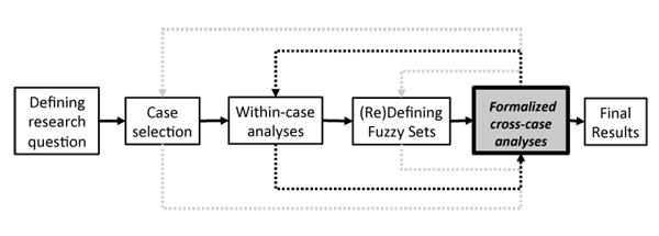
Figure 1: Research process with QCA [10]
It is important to note that the results obtained through formalized QCA analyses do not "prove" causal relations. Rather, they reveal patterns of associations across sets of cases or observations, thereby providing support for the existence of such causal relations (SCHNEIDER & WAGEMANN, 2010, p.412). However, an association might reveal an ontological relation (i.e., two events or factors are linked because one constitutes what the other is, rather than causing it; GOERTZ & MAHONEY, 2005) or a spurious causal link (i.e., two events or factors are associated because they are both caused by a third, unobserved factor; e.g., BRADY, 2008, p.229). Hence, whether it makes sense to interpret associations as causal relations depends on the insights derived from within-case analyses, as well as existing empirical and theoretical knowledge of the phenomenon under investigation (BLATTER, 2012, p.3; GEORGE & BENNETT, 2005, pp.206f.). [11]
In short, QCA does not work as a "push-button" process, but relies on the copious efforts of the users to reflect on whether identified patterns could describe a causal link (RIHOUX, 2009a, p.368; SCHNEIDER & WAGEMANN, 2010, p.410). Henceforth, when I refer to necessary or sufficient conditions being "identified" by QCA, I refer to the respective patterns of association and assume that they make theoretical and empirical sense as such conditions. [12]
QCA offers many benefits for qualitative researchers: a unique set of tools for tackling research questions that are based on set-theoretic notions and for analyzing causal complexity; a boost in analytic potential for cross-case comparisons that is especially useful for medium-N data sets; help in making research more systematic and transparent; and insights into causal and/or typological patterns that assist the development of mid-range theories. [13]
First, many theoretical models and research questions in the social sciences, at least implicitly, draw on set-theoretic notions by assuming that there are conditions that are necessary or sufficient for the occurrence of a given phenomenon (GEORGE & BENNETT, 2005, p.212; RAGIN, 2008, p.13; WAGEMANN & SCHNEIDER, 2010, p.380; for an explanation of the notions of necessity and sufficiency, see below). Moreover, just as set-theoretic notions underlie much of social science thinking, many social phenomena can and should be understood as instances of complex causality. In most cases, factors that influence the occurrence of an event or phenomenon do so in conjunction. Different combinations are able to lead to a given event or phenomenon, and factors can have differing effects depending on the situation they work in (LIEBERSON & LYNN, 2002; RAGIN, 2008, pp.23-25, 177f.). QCA offers the most systematic way to analyze complex causality and logical relations between causal factors and an outcome (SCHNEIDER & WAGEMANN, 2007, p.41). [14]
Second, QCA's potential for systematic cross-case comparison is especially helpful for qualitative researchers working with medium-N data sets (about fifteen to 50 cases). If researchers are interested in what produces a certain event or phenomenon (causality), or want to know what different variants of a given phenomenon exist (typology), QCA provides the unique possibility to combine classic in-depth qualitative analysis with systematic cross-case comparisons. It identifies patterns as well as cases deviating from these patterns using clear logical operations. Its formal language provides a useful way to convey a study's central findings to the reader or audience. In short, QCA helps qualitative researchers to handle the considerable amount of data of a medium-N case study, both during the analytical process and when presenting the findings. [15]
Third, the described systematization and formalization of the QCA research process entails a number of advantages for qualitative researchers. For one thing, it increases the transparency of analyses by making explicit a number of choices researchers have to face, e.g., regarding their concept formation and the use of counterfactual analysis (EMMENEGGER, 2010, p.10; RAGIN, 2008, p.167; RIHOUX, 2009a, p.369). Such transparency makes data analysis and findings more retraceable for the reader, which increases the persuasiveness of argumentation and is a characteristic of good (qualitative) research (GEORGE & BENNETT, 2005, p.70; KING, KEOHANE & VERBA, 1994, p.26). For another, by formalizing concepts as conditions and assigning membership values to the cases, QCA helps to focus the attention on key issues of conceptualization and helps to detect blurry or problematic aspects in conceptualizations that might have been overlooked otherwise (GOERTZ, 2006a, pp.37, 101). [16]
Lastly, QCA allows identifying patterns in the data that help to guide the development of detailed explanations of social phenomena. By pointing to the different (combinations of) conditions that can produce an outcome, the method helps abstracting from the idiosyncracies of single cases and developing comprehensive accounts of these phenomena. Through the iterative refinement of these accounts using a close dialogue between detailed within-case analyses and formalized cross-case comparisons, QCA is a powerful tool for the development of cutting-edge mid-range theories. [17]
Despite its many merits, the usefulness of QCA depends largely on the type of research one wishes to conduct. In small-N studies, QCA cannot be employed because the method requires a minimum number of cases (approximately ten cases). Also, for certain research interests the method's focus on complex causality and identifying combinations of conditions might not be helpful (e.g., hermeneutic approaches in which the individual production of meaning is the focus of attention). Thus, as with all research methods, whether it makes sense for a researcher to employ QCA ultimately depends on his or her research. [18]
In this second part of the article, I will introduce the main concepts underlying QCA: the notions of sets and the relations of necessity and sufficiency; consistency and coverage as parameters of fit; the truth table as a central tool for data analysis; the process of minimization; and the different solution terms offered by QCA. Understanding these concepts is a prerequisite for using QCA in a meaningful way because they help to understand what is going on during the analysis and provide the basis for interpreting the results. [19]
3.1 Fuzzy sets and necessity and sufficiency
Fuzzy set QCA uses (fuzzy) set theory and Boolean algebra to analyze formally to what degree certain factors or combinations of factors are present or absent when a phenomenon of interest occurs or fails to occur. In QCA terms, factors that are thought to be causes of a phenomenon are called "conditions," while the phenomenon itself is called "outcome." Factors can be causally linked to an outcome as necessary or sufficient conditions, either by themselves or in combination with one another. In order to formalize the analysis of such conditions, QCA uses the corresponding set-theoretic relations of supersets and subsets, respectively, and Boolean algebra to operate with different sets. In the following section, these basic notions are introduced. [20]
3.1.1 Sets, conditions and outcomes, and Boolean operations
Sets can be understood as formalized representations of concepts. Cases can be evaluated in terms of their membership in such sets. To do so, cases are first analyzed using a preferred qualitative analytic technique (e.g. BLATTER, 2012; GEORGE & BENNETT, 2005, pp.205ff.; GERRING, 2007, pp.172ff.; MAHONEY, 2012; STRAUSS & CORBIN, 1998). After this initial analysis, the researcher should have identified a set of conditions that he/she expects to lead to the outcome, and he/she should have constructed concepts that can capture these conditions. Based on the acquired case knowledge, the researcher can now assign fuzzy membership scores in the different conditions and the outcome to the cases. (For a guide to constructing concepts that are easily translatable into fuzzy sets, see GOERTZ, 2006a; for an explanation of how to code data to assign membership scores to fuzzy set conditions based on qualitative data, see BASURTO & SPEER, 2012.) This comprises the first step of formalization and preparing the data for QCA. [21]
Fuzzy set membership scores range from 0 to 1 and are able to describe differences both in degree and kind of membership of cases in a set. Three anchor points define a set: full membership (indicated by a membership score of 1), full non-membership (membership score of 0), and a crossover point (membership score of 0.5).3) Between the extremes of full membership and full non-membership, a set can have more or less fine-grained membership levels, ranging from four-level sets (e.g., 0, 0.33, 0.67, and 1) to continuous sets (where the fuzzy score can take any value between zero and one). Cases on different sides of the crossover point are qualitatively different, while cases with differing memberships on the same side of the crossover point differ in degree (RAGIN, 2008, pp.72ff.). [22]
Thus, in a hypothetical data set on social upward mobility, every case could be assigned a score reflecting its membership in the set of "social upward mobility" as well as causal conditions expected to influence the outcome (e.g., "social capital" or "government support").4) In order to assign membership scores to cases, one needs to 1. define criteria for assigning membership scores, specifying the qualitative anchors as well as each specific membership level; and 2. know the cases in question in order to make an informed decision about membership.5) [23]
In order to analyze data on the basis of the assigned set membership, QCA draws on Boolean algebra. Using Boolean algebra for QCA, three basic operations can be applied to fuzzy sets: intersection, union, and negation. Figure 2 gives an overview over these operations. (The dashed areas in the graphics demarcate the result of the respective operations.)
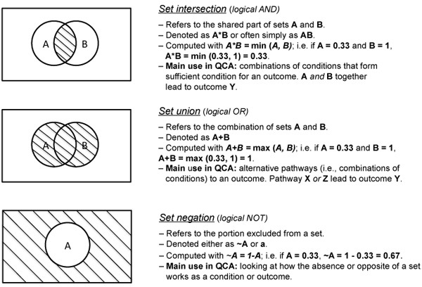
Figure 2: Boolean operations relevant for QCA [24]
Set intersection (logical AND, "*") is the operation that is used to assess a case's membership score in a combination of conditions such as the causal recipes identified through formalized QCA (see below). Set union (logical OR, "+") is the operation that is used to assess the membership score in alternative conditions for a given outcome; e.g., the different causal recipes identified by QCA are connected via logical OR because they are alternative pathways to the outcome (see below). Set negation (logical NOT, "~") is used to include the absence of a condition or an outcome in the analysis. In the actual analysis, software will do all computing of set operations. Still, it is important to understand the basic logic behind those operations and the notations used to describe them. [25]
3.1.2 Set relations: Necessity and sufficiency
The goal of QCA is to identify conditions or combinations of conditions that are necessary or sufficient for the outcome. While QCA operates with the corresponding set-theoretic concepts of supersets and subsets, respectively, for simplicities sake I will only use the logical terms of necessary and sufficient conditions.6) In the following section, these concepts are introduced. [26]
Condition A is necessary for outcome Y if the occurrence of Y is not possible without the presence of A, but A alone is not enough to produce Y. In such cases, all cases in which outcome Y occurs share the presence of condition A. In fuzzy set terms, a necessary relation exists if outcome Y is a subset of causal condition A; that is, in each case the degree of membership in Y is less than or equal to the degree of membership in A (Y ≤ A). As Figure 3 illustrates using fictive data, one can visualize necessity in two ways: Venn diagrams and XY plots. 1. Using a Venn diagram, the circle representing outcome Y is completely engulfed by the (larger) circle representing condition A; there are cases included in set A that are not in set Y, but all cases in set Y are also in set A. 2. XY plots in the context of QCA work differently from their logic in the context of regression analysis. Plotting causal condition A against outcome Y, if all cases fall on or below the main diagonal (sprinkled area), this indicates necessity. Cases falling above the main diagonal (striped area) contradict necessity. As both illustrations show, cases in which A is present but Y is not are not in contradiction with necessity. [27]
Figure 3 also shows the same visualizations for the relation of sufficiency. A condition A or combination of conditions X is sufficient for outcome Y if Y will always occur if A is present, but other conditions besides A that may also produce Y. Empirically, this means that all cases where A is present share the occurrence of Y. In fuzzy set terms, a sufficient relation exists if A is a subset of outcome Y; that is, across all cases the degree of membership in condition A or combination of conditions X is consistently less than or equal to the degree of membership in outcome Y (A ≤ Y). Visualized as a Venn diagram, the circle representing condition A is completely engulfed by the (larger) circle representing outcome Y. When A is plotted against Y, all cases on or above the main diagonal indicate sufficiency, while cases below the main diagonal challenge sufficiency. As both illustrations show, cases in which Y occurs but A is not present are not in contradiction with sufficiency.
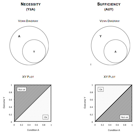
Figure 3: Visualizations of logical relations [28]
QCA helps to identify different empirical patterns that can be interpreted in terms of necessity and sufficiency. These patterns can include one or several single conditions, but also combinations of two or more conditions. In empirical reality, one will usually find combinations of conditions being sufficient for an outcome rather than single ones (GOERTZ & LEVY, 2007, p.22). In such cases, the single conditions that form part of the combination are "INUS" conditions7); they are neither necessary nor sufficient by themself, but part of one or more of the combinations of conditions that are sufficient for outcome Y. [29]
Expressed in set-theoretic terms, the combination of two or more conditions is more likely to be sufficient for an outcome because sufficiency is defined as X ≤ Y and combinations of conditions are computed by taking the minimum of the membership values (A * B = min (A, B), see above). Thus, if X is a combination of the conditions A, B, and C, each case's membership in X will always be smaller than or equal to its membership in the individual conditions. [30]
3.2 Parameters of fit in QCA: Consistency and coverage
In real data, conditions or combinations of conditions in which all cases conform to a relation of necessity or sufficiency are rare; at least a few cases will usually deviate from the general patterns. Therefore, it is important to be able to assess how well the cases in a data set fit a relation of necessity or sufficiency. In QCA, two central measures provide parameters of fit: consistency and coverage (RAGIN, 2006, 2008, pp.44ff.). [31]
"Consistency" measures the degree to which a relation of necessity or sufficiency between a causal condition (or combination of conditions) and an outcome is met within a given data set (RAGIN, 2006). It resembles the notion of significance in statistical models (THIEM, 2010, p.6). In most cases of QCA studies, conditions or combinations of conditions are "quasi-necessary" or "quasi-sufficient" in that the causal relation holds in a great majority of cases, but some cases deviate from this pattern. RAGIN (2006) introduced a formula based on which the fs/QCA software computes consistency scores. Consistency values range from "0" to "1," with "0" indicating no consistency and "1" indicating perfect consistency. [32]
Once it has been established that a condition or combination of conditions is consistent with necessity or sufficiency, coverage provides a measure of empirical relevance. The analogous measure in statistical models would be R2, the explained variance contribution of a variable (THIEM, 2010, p.6). Coverage is computed by gauging "the size of the overlap of [...] two sets relative to the size of the larger set" (RAGIN, 2008, p.57), with values again ranging between "0" and "1." [33]
3.3 Representing cases as configurations of conditions: Truth tables and limited diversity
The truth table analysis serves to identify causal patterns of sufficiency; combinations of conditions ("causal recipes," see below) that are sufficient for the outcome. It builds on the truth table, a distinct way of representing the cases in a data set as configurations of conditions. Table 1 shows a truth table with three conditions A, B, C, as well as the outcome Y. Each condition and the outcome are represented in a column in the truth table. Additional columns show how many empirical cases show a particular configuration ("Cases"), whether the cases agree in displaying the outcome ("Outcome Y"), and what a configuration's level of consistency with sufficiency is ("Consistency").
|
|
A |
B |
C |
Cases |
Outcome Y |
Consistency |
|
I |
1 |
1 |
1 |
1 |
1 |
1.00 |
|
II |
1 |
1 |
0 |
4 |
0 |
1.00 |
|
III |
1 |
0 |
1 |
2 |
1 |
1.00 |
|
IV |
0 |
1 |
1 |
0 |
? |
? |
|
V |
1 |
0 |
0 |
1 |
0 |
0.00 |
|
VI |
0 |
1 |
0 |
3 |
0 |
0.33 |
|
VII |
0 |
0 |
1 |
0 |
? |
? |
|
VIII |
0 |
0 |
0 |
1 |
0 |
0.00 |
Table 1: Exemplary truth table (hypothetical data) [34]
In a truth table, all logically possible configurations of a given set of conditions are displayed. For instance, Row I represents cases where all three conditions are present (indicated by "1" in the respective column) while Row VIII represents cases where all conditions are absent (indicated by "0"). In this fashion, each configuration is represented as a row in the truth table. A truth table has 2k rows, with k being the number of causal conditions included in the model.8) [35]
Having assigned membership scores to the cases for each fuzzy set, one can compute which configuration of conditions best represents each case in the data set (each case will always belong to exactly one configuration). By looking at whether the case(s) assigned to a truth table row agree in displaying the outcome (indicated by the consistency column), the researcher can assess whether a given configuration of conditions can be regarded as sufficient for the outcome.9) [36]
Practically all empirical phenomena are limited in their variation and tend to cluster along certain dimensions; a characteristic that has been coined "limited diversity" (RAGIN, 1987, pp.106-113). Limited diversity is virtually omnipresent in sociological research and poses a problem for small-N as well as for large-N data sets (RAGIN, 2008, p.158; SCHNEIDER & WAGEMANN, 2007, pp.101-112). In QCA, limited diversity manifests itself in that some truth table rows will usually remain empty, i.e., no empirical cases that belong to these rows are contained in a data set (e.g., Rows IV and VII in Table 1). These empty rows are called "logical remainders." Being able to identify logical remainders and thus making limited diversity visible is a distinct strength of QCA. In the following section, I will explain how logical remainders play a role in QCA and how simplifying assumptions help to address the problem of limited diversity. [37]
3.4 Boolean minimization and simplifying assumptions
The QCA software looks at the distribution of cases over the truth table rows and checks whether cases belonging to the same configuration display the outcome. Thereby, it identifies the basic configurations of conditions that are sufficient for the outcome, the so-called "primitive expressions." In Table 1, the primitive expressions that are consistent with being sufficient or Outcome Y are ABC (row I) and AB~C (row III). Such terms are precise descriptions of conjunctions of conditions that are sufficient for the outcome; often, however, they are quite complex because models include more than just three causal conditions. QCA uses "Boolean minimization" to reduce the primitive expressions and arrive at intelligible solutions.10) In practice, software packages conduct the minimization (e.g., in the form of the truth table analysis tool in fs/QCA). In this section, I will explain the basic notions behind this process that are necessary to operate the software and understand what it is doing. [38]
Using the primitive expressions that were identified as sufficient in the truth table, Boolean minimization serves to identify more and more general combinations of conditions sufficient for the outcome that remain logically true. One way this process works is by focusing on pairs of configurations that differ in only one combination but agree in displaying the outcome. Take the primitive expressions from Table 1: both ABC and AB~C consistently show the outcome. In such a case, the presence or absence of C does not influence the occurrence of the outcome Y (SCHNEIDER & WAGEMANN, 2007, pp.63-73). This reduces primitive expressions to simpler combinations of conditions; e.g., ABC ≤ Y and AB~C ≤ Y are simplified to AB ≤ Y. As the end product of this minimization process, QCA identifies "causal recipes"—combinations of conditions that are generalizations of the patterns that exist in the data set and are minimized in their complexity. [39]
From an analytic perspective, the value of these causal recipes lies in containing the "story of the cases." They describe the patterns in the data set. However, they are not the story; as mentioned earlier, in order to really understand what they are describing and produce lucid explanations of the outcome, the researcher has to go back to analyze the cases, using the causal recipes provided by QCA as an analytic lens (see below for suggestions of how to execute such analyses). [40]
Due to limited diversity, it is often hard to find pairs that differ on only one condition and agree in displaying the outcome. To continue the minimization process, RAGIN (2008, pp.145-175) suggests the use of simplifying assumptions. Simplifying assumptions are theory-driven assumptions of how a given condition might be causally related to the outcome. [41]
Simplifying assumptions are based on counterfactuals; thought experiments in which the researcher theorizes about how an event or phenomenon would have unfolded had a given causal condition been different. For tackling the problem of limited diversity in QCA, the researcher uses simplifying assumptions to theorize about whether a given configuration of conditions not present in the data set would display the outcome or not.11) [42]
Hence, using simplifying assumptions in the minimization process can be more or less problematic depending on the amount of theoretical and substantive knowledge the researcher brings to the table (for critiques of this practice and answers to these critiques, see DE MEUR, RIHOUX & YAMASAKI, 2009; RAGIN, 2008, pp.147-175; SCHNEIDER & WAGEMANN, 2007, pp.105-109). To assess when a simplifying assumption is legitimate, RAGIN and SONNETT (2005) introduce the notion of "easy counterfactuals" as those cases in which substantive empirical or theoretical knowledge gives a clear notion of how a condition contributes to an outcome (i.e., when present or absent). In such cases, the researcher is able to formulate a directional expectation of how the condition could be related to the outcome, which serves as a simplifying assumption. If empirical or theoretical knowledge is lacking or suggests that the presence and absence of a condition could contribute to an outcome, one should refrain from using simplifying assumptions. Thus, the researcher should formulate a compelling counterfactual every time he/she uses a simplifying assumption, and he/she should make this decision explicit when presenting findings (for criteria of good counterfactuals, see EMMENEGGER, 2010). This transparent and straightforward way to address the problem of limited diversity is a major strength of QCA as an analytic technique (RAGIN, 2008, p.155).12) [43]
3.5 Complex, parsimonious, and intermediate solutions
Depending on the approach to simplifying assumptions in fs/QCA, the truth table analysis (TTA) yields three different solution terms: 1. complex, 2. parsimonious, and 3. intermediate solution13) (RAGIN, 2008, pp.148-150). The causal recipes contained in these solution terms may differ more or less from each other, but they are always equal in terms of logical truth and never contain contradictory information. [44]
The complex solution does not allow for any simplifying assumptions to be included in the analysis. As a result, the solution term is often hardly reduced in complexity and barely helps with the data analysis, especially when operating with more than a few causal conditions. The parsimonious solution reduces the causal recipes to the smallest number of conditions possible. The conditions included in it are "prime implicants," i.e., they cannot be left out of any solution to the truth table. The decisions on logical remainders are made automatically, without regard to theoretical or substantive arguments on whether a simplifying assumption makes sense. RAGIN (2008, pp.154ff.; see also SCHNEIDER & WAGEMANN, 2007, pp.106f.) argues strongly against such a use of simplifying assumptions. Finally, the intermediate solution includes selected simplifying assumptions to reduce complexity, but should not include assumptions that might be inconsistent with theoretical and/or empirical knowledge. It can be understood as the complex solution reduced by the conditions that run counter to fundamental theoretical or substantive knowledge (SCHNEIDER & WAGEMANN, 2012, p.172). [45]
In practice, fs/QCA computes the complex and parsimonious solutions regardless of simplifying assumptions, whereas the intermediate solution depends on the specifications of simplifying assumptions. The viability of the intermediate solution thus hinges on the quality of the counterfactuals employed in the minimization process. Given a diligent use of simplifying assumptions, the intermediate solution is recommended as the main point of reference for interpreting QCA results (RAGIN, 2008, pp.160-175). [46]
In the first two parts of this article, I introduced the main principles and concepts underlying QCA. With these principles and concepts as the basis, in the following two parts I will turn to the practical use of the method, looking at the applications of QCA's analytic tools and the incorporation of QCA results into data analysis. [47]
4. Analytic Tools of QCA and their Applications
QCA's analytic tools are applied in the formalized cross-case comparisons of the QCA research process. Before this stage, the researcher should have acquired in-depth knowledge of his/her cases through detailed within-case analysis. Any analytic method that focuses on a qualitative, in-depth analysis of cases can be used for this step of the research process. For instance, the within-case analysis can focus on causal processes and the identification of mechanisms (e.g., BLATTER, 2012; GEORGE & BENNETT, 2005, pp.205ff.; GERRING, 2007, pp.172ff.; MAHONEY, 2012) and/or on the construction of concepts and typologies (e.g., STRAUSS & CORBIN, 1998). For a description of how to calibrate qualitative data (i.e., develop rules to assign membership scores to fuzzy set conditions based on qualitative data), see BASURTO and SPEER (2012). [48]
It is always recommended to use one of the available software packages to conduct a QCA. Among the software packages for fuzzy set QCA, fs/QCA (RAGIN & DAVEY, 2009) is the most widely used option. It is a freeware program that allows both crisp and fuzzy set analyses, provides a function to produce an intermediate solution, as well visualizations such as XY plots. As a further plus, it does not require computation commands, but runs with a graphical user interface. In the following discussion, I will focus on practical applications and tips for analytical tools provided by this software.14) [49]
Having finished the within-case analysis, the first step of cross-case comparison should always be to get an overview of the data set. There are different tools at hand to do so: basic descriptive statistics, XY plots, and the truth table. In the following section, I will provide suggestions for how to use each of these tools in the analysis. [50]
The descriptive statistics functions in fs/QCA are tools to gain a quick overview over a data set's conditions and the outcome category. The descriptive statistics tools are useful mainly to gather first impressions of a data set. These impressions help to reflect upon how fuzzy membership scores were assigned, implement changes if warranted, and track these changes in the data. For instance, using the descriptive statistics function, the researcher can check whether the mean membership in the outcome is very low, which would indicate that the outcome is rarely present in the data set. If this is the case, it is relatively easy for conditions to be consistent with necessity (because necessity: Y ≤ A), but it will be difficult to find any sufficient conditions (because sufficiency: Y ≥ A). Conversely, if mean membership in the outcome is very high, it is relatively easy for single conditions to be consistent with sufficiency, but there will not be any necessary conditions to be found. Following the same logic, a condition with a very high mean membership score might well be necessary; a condition with very low membership will often be sufficient. [51]
Finding such extreme mean membership scores is not problematic in itself, but it might indicate that the coding of a given condition or outcome does not capture relevant variation. For instance, looking at social mobility, if one only defines cases of "from rags to riches" as "upward mobility" (membership in the set of social mobility of 1.0) and draws the data set from a random primary school class, most respondents will have very low membership in the outcome, possibly leading to a number of conditions being necessary for such extraordinary upward mobility. While this might make theoretical sense, one could also argue that such an extreme definition misses important variation. It might prove more fruitful to define upward mobility more moderately in order to capture in more detail the kind of moderate upward mobility that is a more common social phenomenon. If this is the case, changing the coding scheme for this condition or outcome might be an option. However, this step needs to be carefully reflected upon and should not be motivated by the need to find some kind of association in the data. Changes should only be pursued if they make theoretical sense (SCHNEIDER & WAGEMANN, 2010, p.405). Using the frequencies function, one can compare the distribution of cases along a given condition with the old and new coding scheme, thus keeping track of how strongly the changes made affect this distribution. [52]
A very useful exploratory tool is the XY plot (SCHNEIDER & GROFMAN, 2006, pp.36-39; SCHNEIDER & WAGEMANN, 2007, pp.197ff.). First, the XY plot serves as a tool for quick inspection of set relations between causal (combinations of) conditions and the outcome. Before running a truth table analysis (see below), it helps to get an overview of how single causal conditions and the outcome might be related. Getting such a first idea of patterns in the data comprises an important step in any data analysis (SCHMITTER, 2008, p.287). [53]
Second, the XY plot comprises an intuitively accessible visualization of set relations. If all or almost all cases fall above the main diagonal, this indicates a sufficient relation. If all or almost all cases fall below the main diagonal, this suggests a relation of necessity. XY plots also visualize coverage: the further cases fall away from the main diagonal, the lower the coverage (RAGIN, 2008, p.60). Thus, the prospective reader can get an idea of causal patterns in a data set.15) [54]
Third, the XY plot indicates whether necessary or sufficient relations exist between some of the causal conditions. If indications exist that a causal condition could be a necessary or sufficient condition for another causal condition in the model, such information has theoretical value and helps to further the knowledge of causal patterns in the cases. As a consequence, the researcher might decide to drop a given condition or conflate two conditions if it makes theoretical sense to do so. For instance, say a study tries to explain students' school performances and includes students' educational expectations as well as the parents' expectations as conditions. A quick look at the relation between these two conditions might reveal that parents' high expectations were a sufficient condition for high student expectations. In such a case, one could use this insight for further within-case analysis, focusing on how parents influence students' expectations and introduce a new condition into the QCA model instead of the two conditions used before. [55]
Finally, scrutinizing XY plots helps identifying deviant cases in the data set and investigating what type of inconsistencies they might be: inconsistencies in degree or in kind16) (see SCHNEIDER & WAGEMANN [2012, pp.126f., 306-308] for an explanation of how to identify different types of inconsistent cases). This analytic step is important because 1. the type of inconsistency a deviant case represents informs about how seriously it calls a relation of necessity or sufficiency into question; and 2. identifying and analyzing deviant cases helps to deepen the knowledge of the causal patterns in a data set and refine the conceptualizations and model specification. Sticking with the above example, it would be helpful to identify cases that deviate from the pattern "parents' high expectations are sufficient for students' high expectations." Such deviant cases might reveal that expectations are not transmitted if there is no relationship of trust between parents and child. This insight could lead to a further refinement of the condition in question, and also provide further hints for what aspects to focus on in the within-case analysis: how parents and child build trust between each other, and how this in turn affects the transmission of educational expectations. [56]
4.1.3 Working with the truth table
The truth table includes much information, as it is a complete representation of patterns in the data. Therefore, it is important to scrutinize the truth table before continuing with the truth table analysis (SCHNEIDER & GROFMAN, 2006, p.13; SCHNEIDER & WAGEMANN, 2010, p.406). One important step is to look for truth table rows whose configurations have high, but not perfect consistency scores. It is fruitful to analyze the cases deviating from the general pattern more closely and try to figure out whether one overlooked an important condition or aspect of an existing condition; this might help to clear up the inconsistency and improve the model and understanding of the cases, as illustrated in the example above. [57]
Another step is to reflect on the distribution of cases and assess the extent of limited diversity (SCHNEIDER & WAGEMANN, 2010, pp.406f.): Are there logical remainders, i.e., truth table rows that are not populated by any case (check the [number] column)? Is there an explanation for why these truth table rows remained empty? Which, if any, rows are populated with a relatively large number of cases? Answering these questions reveals much about the nature of the phenomenon under investigation and shows the extent and nature of limited diversity in the data set. [58]
Again consider the example of students' school performance. Checking the truth table for logical remainders might reveal that all truth table rows remained empty that combined the absence of the condition "trust between parents and child" with the presence of the condition "emotional support from parents," and vice versa. This insight would tell something about the nature of limited diversity in the data set. One could argue that this particular set of logical remainders stems from this configuration (no emotional support from parents, but trusting relationship between parents and child, or vice versa), not existing in empirical reality (see SCHNEIDER & WAGEMANN, 2007, pp.101ff., for this and other types of limited diversity). Furthermore, it would suggest reconsidering conceptualizations and model specification, because "emotional support from parents" and "trust between parents and child" seem closely related phenomena that might be conflated into one condition. [59]
A look at the truth table might also provide first indications of the special importance of specific conditions. For instance, only students who received emotional support from their parents could show high school performance. In the truth table, this pattern would show by only rows with the condition "emotional support from parents = 1" displaying the outcome. Such insights point to possible foci for further within-case analysis. [60]
As mentioned above, one should test what conditions might be necessary for the outcome before analyzing sufficiency. Some important aspects when using QCA tools to identify necessary conditions are consistency thresholds and empirical relevance, theoretical reflections on identified conditions, and reflections on research questions and coding schemes. [61]
When testing conditions for their necessity, remember that the threshold for consistency should be high (> .9) and its coverage should not be too low (> .5). Identifying a necessary condition is quite rare empirically. Claiming a condition was necessary for an outcome is a rather bold statement and such relations are in fact rarely to be found empirically (GEORGE & BENNETT, 2005, pp.26f.; SCHNEIDER & WAGEMANN, 2007, pp.41, 60). Hence, finding multiple necessary conditions might indicate that the mean membership in the outcome is very low (see above). In such cases, there might be theoretical grounds for recalibrating the outcome set. [62]
The truth table analysis (TTA) is the core element of the formal data analysis with QCA. It consists of 1. converting fuzzy sets into a truth table and 2. minimizing the sufficient configurations in the truth table to more parsimonious causal recipes. The software handles the above operations.17) In this section, I will 1. explain how to read and interpret the TTA output, and 2. suggest the creation of an enhanced table of QCA results. [63]
4.3.1 How to read and interpret truth table analysis output
The output of the TTA consists of the complex, the parsimonious, and the intermediate solution. As explained above, in the interpretation of the results the intermediate solution will usually be the main focus. Hence, in my discussion I focus on this part of the output.
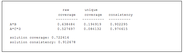
Figure 4: Exemplary output of truth table analysis (abridged) [64]
The table in Figure 4 contains the vital information of the output. To the left, the causal recipe(s) are listed that remain after the minimization procedure. They are the combinations of conditions that comprise alternative sufficient paths to the outcome. The first column shows the raw coverage of each recipe, that is, the extent to which each recipe can explain the outcome. The second column displays the recipes' unique coverage, i.e., the proportion of cases that can be explained exclusively by that recipe. Finally, the third column shows each recipe's consistency score. Below the list of causal recipes is the solution consistency and coverage. Solution consistency indicates the combined consistency of the causal recipes. Solution coverage indicates what proportion of membership in the outcome can be explained by membership in the causal recipes. [65]
While the researcher should always develop substantive interpretations of formalized QCA results in dialogue with the data (see below), some general guidelines can be given. First, if consistency is below 1.0, this means that the recipe covers one or more cases that do not display the outcome; i.e., they deviate from the general pattern found in the data. The lower a consistency score, the more cases do not fit the patterns identified by QCA, or the more substantial are the contradictions that certain cases pose. For instance, in the output shown in Figure 4, the recipe AB (.90) has a considerably lower consistency score than recipe ACD (.97). A first step could be to investigate whether these are inconsistencies in degree or in kind. A convenient way to examine this is to use SCHNEIDER and WAGEMANN's approach (2012, pp.126f., 306-308) and use XY plot functions such as the one provided by fs/QCA to visualize the relation between the causal recipe and the outcome. The researcher should note for each recipe how many cases are inconsistent in total, and how many of these are inconsistent in degree and kind. Finding one or several cases that are inconsistent in kind casts substantial doubt on the causal claim of sufficiency underlying that recipe. [66]
Regarding the raw coverage of recipes, the lower a coverage score, the less empirically relevant a causal recipe; it is able to explain fewer cases in which the outcome occurred. Figure 4 shows that recipe AB (.64) has a higher raw coverage score than ACD (.53), indicating that the former covers more cases in the data set. One approach to the results is to start with the recipe showing the highest raw coverage as the main recipe. One can compare the recipe's raw coverage to the solution coverage, or compare whether the recipe also has the highest unique coverage or whether some other recipe has a higher score in this regard. Because of how coverage is computed (see RAGIN, 2006), differences in coverage scores not always reflect differences in absolute numbers of cases. Hence, it might help with the interpretation and presentation of the findings to translate the coverage scores into absolute numbers. To do so, look at which cases are members of which recipes and note the total number and case ID of those cases that are members of a given recipe (the fs/QCA software provides a useful tool for this; see Appendix 1). [67]
The unique coverage scores can be used for two interrelated observations: cases uniquely explained by a recipe and overlap between recipes. First, unique coverage is meaningful because it indicates how many cases a given recipe can explain without any other recipe offering explanation. Recipes with higher unique coverage thus gain relevance because without them more cases would be beyond the explanatory reach of the model. As above, it helps to note the absolute number of cases uniquely explained by each recipe. Second, often there is considerable overlap between recipes, so it is not unusual for the unique coverage scores to be rather low (< .15). The degree of overlap can be computed by subtracting the sum of unique coverages from the solution coverage (GLAESSER, 2008, p.201); the absolute number of overlapping cases can be derived by checking case membership in the different recipes as explained earlier. In the above example, the overlapping coverage is .44, or nine cases. The extent of overlap indicates two things. On the level of the data set, it shows how strongly the cases cluster along certain dimensions on the causal conditions. On the level of the single cases, it shows in how many cases with the occurrence of the outcome can be explained in more than one way. [68]
If consistency and/or coverage scores for the solution are low (below .75), this indicates a badly specified model. Problems might derive from including irrelevant conditions and/or missing crucial conditions, using inadequate indicators, or miscalibrating conditions or the outcome. Looking at the output in Figure 4, the solution coverage of .72 suggests that a substantial number of cases (six cases, in absolute numbers) where the outcome is present are not a member of any recipe and can thus not be explained by the model. To identify which cases are not member of any recipe and thus remain unexplained, compute a new condition that combines all recipes via logical OR and plot this condition against the outcome in an XY plot (see Appendix 1 for a technical description). All cases with membership in the new "solution" condition below 0.5, but with membership in the outcome higher than 0.5, are unexplained cases (they will be located in the upper left quadrant of the plot). [69]
4.3.2 Enhanced table of QCA results
Based on these first interpretations, it is helpful to create an enhanced table of QCA results. This table may include: 1. the recipes and their parameters of fit (i.e., consistency, raw coverage, and unique coverage); 2. solution parameters; 3. the extent of limited diversity as the proportion of logical remainders over the total number of truth table rows (as derived from the analysis of the truth table, see above); 4. simplifying assumptions specified; 5. the absolute number of cases inconsistent with a recipe overall, in degree, and in kind; 6. the absolute number of cases that are members of each recipe and the solution; 7. a list of the cases that are members of the recipes (using a case ID or abbreviation); 8. the extent of overlap in the solution, in terms of absolute number and proportion; 9. the overall absolute number and proportion of uniquely covered cases; and 10. a list of cases with the outcome present that are not members of any recipe in the solution. Based on the TTA from Figure 4, this would yield the following table:
|
|
Recipe 1: A*B |
Recipe 2: A*C*D |
|
Consistency |
0.90 |
0.97 |
|
… # of incons. cases |
5 |
1 |
|
… in degree |
4 |
1 |
|
... in kind |
1 |
0 |
|
Raw coverage (# of cases) |
0.64 (16) |
0.53 (13) |
|
Unique coverage (# of cases) |
0.19 (7) |
0.08 (4) |
|
ID of cases explained |
1, 5, 6, 10, 13, 14, 15, 18, 20, 21, 23, 27, 31, 32, 33, 34 |
5, 6, 11, 14, 15, 17, 20, 21, 22, 31, 32, 34, 38 |
|
ID of cases explained uniquely |
1, 10, 13, 18, 23, 27, 33 |
11, 17, 22, 38 |
|
Solution parameters |
|
|
|
Consistency |
0.91 |
|
|
… # of incons. cases |
5 |
|
|
… in degree |
4 |
|
|
… in kind |
1 |
|
|
Coverage (# of cases) |
0.72 (20 cases) |
|
|
Unique coverage (# of cases) |
0.28 (11 cases) |
|
|
Overlap (# of cases) |
0.44 (9 cases) |
|
|
# of unexplained cases (case ID) |
6 cases (9, 12, 16, 24, 30, 37) |
|
|
Limited diversity |
62.5 per cent (10 of 16 truth table rows covered) |
|
|
Simplifying assumptions |
Condition A (present) Condition B (present) Condition C (present) Condition D (present) |
|
Table 2: Enhanced table of QCA results [70]
Such a table combines the results from the formalized QCA with additional information. It provides a comprehensive, concise representation of the outcome that can serve as a point of quick reference when re-analyzing cases in the light of QCA results. [71]
5. Incorporating QCA Results in Data Analysis
Remember that the causal recipes identified by the truth table analysis (TTA) contain the explanation of the outcome, but they are not that explanation. To establish whether a causal relation exists between a set of conditions and an outcome requires two (connected) steps: 1. determine that conditions or combinations of conditions are linked systematically and consistently to the outcome (using the analysis of necessity and TTA tools), and 2. explain how this link works by revealing the underlying mechanisms through subsequent within-case analyses. Thus, having obtained QCA results, a main analytic step still lies ahead: making sense of the cases with the help of the recipes suggested by the TTA and using the cases to find concrete examples of the recipes at work. The crucial step is to check whether QCA results converge with prior and subsequent within-case analyses to produce convincing causal claims. I suggest researchers can approach this dialogue between data and QCA results from three complementary angles: reassessing cases, recipes, and single conditions. These angles build on each other, but the analytic process should not be understood as a linear process from one to the next. [72]
The first angle I suggest is to use QCA results to better understand how the cases work. That is, the researcher reassesses his/her understanding of the cases in the light of the identified causal recipes. Each causal recipe a case is a member of can be seen as a formula for understanding how the outcome came about in that case. The first step is to identify what cases are members of which recipes. For each recipe that covers a case, the researcher should aim to develop a causal explanation of a conjunction or sequence of events that leads to the occurrence of the outcome.18) [73]
Each explanation should recur to the conditions the corresponding recipe includes. For instance, say the recipes AB and AC have been identified as sufficient for the outcome of holding a high-paying job. For instance, AB could describe the combination of having a university degree in engineering (A) AND having extensive weak ties to people working in the field of expertise (B). AC could describe the combination of having a university degree in engineering (A) AND having family who run a business in the field of expertise (C). If A, B, and C are present in a given case, both recipes cover it simultaneously. The researcher can produce a causal account of the case for each recipe, trying to explain the occurrence of having a high-paying job by following the logic of each recipe in turn. In this effort, answering the following questions might be helpful as an orientation:
What are aspects in which the conditions (as they appear in the case) converge with, or diverge from, the general conceptualization? The conceptualizations of certain factors or mechanisms in the form of concepts and causal conditions describe a certain understanding of how these factors or conceptualizations work. The accuracy of these concepts and causal conditions might differ from case to case. It is fruitful to look at whether a given case represents a good example of the general conceptualization, or rather a special instance of a given factor or mechanism. For instance, looking at a case with condition B present (i.e., having extensive weak ties to people working in the field of expertise), one may find that the weak ties helped the respective respondent by providing overall knowledge of how this field of expertise works and what to focus on when applying for a job. However, the conceptualization might have been focused on one or several weak ties taking action directly to help the respondent secure a job.
Is there a discernable temporal order by which the conditions occurred in a case? In some studies, the temporal order in which the conditions occurred in the cases is irrelevant or indiscernible. If it does matter and the data allows scrutinizing this aspect, time constitutes a crucial dimension of case analysis. For instance, knowing the temporal order in which conditions occurred might reveal whether the conditions are interconnected in that one brought about or facilitated the occurrence of another. In some cases a respondent with A, B, and C present might have developed his weak ties to persons working in his field of expertise (B) during his studies independently from his family (C); there is a temporal order in which conditions B and C occurred, but the conditions are not interconnected. In other cases, the family members working in the field of expertise (C) might have introduced the respondent to other people working in the field, thus facilitating the establishment of these weak ties (B); here, a clear causal connection between the conditions B and C exists.
Which recipe covering a given case does the best job in explaining the occurrence of the outcome in that case? Do all recipes seem to lack some component for explaining the case? Often, although several recipes cover a single case, based on detailed knowledge of the case one is able to assess which recipes does the best job of explaining how the outcome came about. For instance, in a case from the above example where A, B, and C are present and the case is thus a member of both AB and AC, the researcher might know that that person is in fact employed in a relative's company. Thus, he/she knows that while the extensive weak ties to the field might also have helped to find a high-paying job in the field of expertise, what actually lead to that person holding a high-paying job was the combination of the university degree in engineering with a family member running a business in the field of expertise. AC thus offers the better explanation of the outcome in this particular case. At other times, the knowledge of the cases might suggest that all the recipes suggested by the TTA that cover a given case do not offer a satisfying explanation of why the outcome came about in that particular case. For instance, though in a case with A, B, and C present, the person might hold a high-paying job outside the field of expertise. Thus, neither AB nor AC seems to offer good explanations of how that person managed to acquire that job. In such cases, the researcher should scrutinize the case in search for further conditions so far omitted from the model in order to improve the explanation of such cases.
Are there cases that cannot be explained by any of the recipes suggested by the TTA? Such cases may exist if the solution coverage is below 1.0. In terms of model fit, this indicates that the model is not able to explain the whole variety of cases in the data set; some ways in which the outcome is produced remain hidden. Again, analyzing such cases in great detail helps to significantly improve the understanding and explanation of the outcome, since it is likely to reveal aspects overlooked so far. [74]
Asking such questions when working with QCA to explore the cases will increase the understanding of the data set as well as the causal recipes identified by the TTA. It will also reveal gaps and inconsistencies in explanations that indicate the need for further in-depth analysis. [75]
A further angle in the dialogue between data and QCA results is to focus on each recipe suggested by the TTA. From this second angle, the guiding question is how recipes work. Taking the insights from reassessing the cases as a starting point, the researcher looks at how well the causal recipes work as more general explanations of the outcome. The goal now is to look at how each recipe works across all cases that are members of it, and to describe their characteristic functioning, or different types of functioning. Parallel to the guiding questions for reassessing cases, the following questions may help when focusing on recipes:
What cases does a given recipe cover, for which of them does it offer the most adequate explanation, and what cases best illustrate the functioning of each recipe? The enhanced table of QCA results already contains the first part of this information (see above). The analyses when reassessing the cases yields information on which cases each recipe describes most adequately.
Across all cases that are members of a recipe, is there a discernable temporal order by which the conditions occurred? Here, the analysis of the temporal order of conditions within cases is informative. It shows whether there are similarities across the cases a given recipe covers. Is there an order in all cases or only in some? Is that order constant across all cases, or does it vary? Are the conditions interconnected in that one brought about or facilitated the occurrence of another?
Does the recipe work in the same way across all cases that are members of that recipe; i.e., does it describe the exact same mechanism, or are different ways discernable in which that recipe seems to work? A good approach to this question is to use the analysis of the temporal order and the assessment of how the different conditions work in each case. Are there different distinct temporal orders discernable in which the conditions in a recipe occur in the cases it covers? Are there different ways discernable in which a condition pertaining to a recipe works in the cases the recipe covers? If a recipe shows different ways in which it works, the researcher can reflect on whether these ways make sense as different types of the same overarching mechanism, or whether he/she is in fact looking at two substantially different mechanisms. In the latter case, the researcher should think about how to revise the conditions and/or model specification in order to reflect this finding and conduct a new round of formalized QCA. Based on this analysis, a further row in the enhanced table of QCA results can indicate for each recipe one or two cases that best illustrate its general functioning. These cases are also crucial when it comes to explaining how each recipe works during the presentation of findings.
Are there certain types of cases the recipe cannot explain satisfactorily? Here, the insights regarding shortcomings in the explanations of the cases based on the recipes identified are helpful. The researcher can try to find patterns in these shortcomings. Maybe a certain recipe has recurring problems with cases that are similar in some relevant aspect, and this insight might help to revise the conditions and/or model specification. Sticking with the above example, one may find that for a certain group of cases that are that are members of the recipe AB (having a university degree in engineering AND having extensive weak ties to people in the field of expertise), the recipe does not seem to offer satisfying explanations. A closer inspection might reveal that in all these cases, the respondent did not in fact activate the resources available through the weak ties in order to secure the job. These cases could have some other aspect in common that still enabled the respondents to secure a high-paying job.
How can deviant cases, i.e. cases that are inconsistent with a recipe, be explained? The researcher already identified the cases that are inconsistent with the recipes when setting up the enhanced table of QCA results. Now he/she should reflect on why they do not work in the way their membership in the recipe suggests. Why does the outcome not occur although all conditions of the recipe are present? Understanding why cases deviate helps to improve the explanations of the outcome, e.g., by introducing a new condition to the model that was overlooked so far. [76]
One further option in reassessing recipes is to look for possibilities to factorize them. Factorizing refers to the merging of similar causal recipes following the rules of Boolean algebra (SCHNEIDER & WAGEMANN, 2012, pp.47-49). For instance, a solution with AB + AC + DE → Y can be merged, yielding A (B + C) + DE → Y. In the merged recipe, A is the condition common to both component recipes, while B and C make up their difference. With rather complex solutions, factorizing can further reduce the complexity of solutions and help their interpretation. [77]
The factorizing of solution terms is, as such, a strictly formal operation, based on the fact that there is some overlap between two or more recipes. What gives this operation substantial meaning is an analysis of what similarities in causal process or characteristics of cases might lie behind this formal overlap. For instance, the condition(s) differing between the recipes could be subsumed under a more general concept. If AB + AC = A (B + C) = Y, identifying a condition F substituting for B and C would lead to AF = Y, with F = B + C. Usually, this substituting concept F will be a more abstract, general one than the concepts C and D it replaces (GOERTZ, 2006a, p.267; GOERTZ & MAHONEY, 2005, p.532). Recurring to the above example of people holding a high-paying job, having relevant ties to people working in the field of expertise (F) might be a more general concept that is present when someone has extensive weak ties (B) OR family who run a business in the field of expertise (C). [78]
5.3 Reassessing single conditions
Lastly, one can approach the dialogue between cases and QCA results from the angle of single conditions.19) This analytic angle, again, draws on the insights gained from the two preceding angles. For one thing, one can analyze a condition substantially, focusing on how it works and what role it plays in the causal explanations developed for the cases. For another, one can reflect on the relative importance of single conditions for producing the outcome in the data set. [79]
Regarding the substantial analysis, the researcher can ask a number of questions that can guide the analysis. Since these questions are similar for single conditions as for the recipes, I will not explain the underlying analytic logic in detail.
Across all cases in which a condition is present, is there a discernable temporal order; i.e., is the condition always preceded or succeeded by a specific second condition? If so, is there a causal link between those conditions?
Does the condition work in the same way across all cases that are members of that recipe; i.e., does it describe the exact same mechanism, or are different ways discernable in which that condition works?
Are there deviant cases, i.e., cases that are inconsistent with how the condition usually works? How can these inconsistencies be explained? [80]
In the course of the substantive analysis, the researcher should pay special attention to conditions that were identified as necessary for the outcome by the formalized QCA. If he/she identified a condition that is consistent with necessity and has rather high coverage (> .5), he/she should ask whether it makes theoretical and empirical sense as a necessary condition. Three questions can help to reflect on this issue: 1. Why should the condition, theoretically speaking, be necessary for the outcome? Does it have some enabling or triggering function without which the outcome is not possible? Or can I easily construct a realistic scenario in which the condition would not be necessary for the outcome, even under the same scope conditions? 2. If the condition is not perfectly consistent with necessity, what is happening in cases that contradict the pattern of necessity? Here, the same close scrutiny applies as with cases inconsistent with the sufficiency of causal recipes (see above). And 3. are there cases in the data set that are consistent with the pattern, but where it would be plausible to argue that the outcome would also have occurred with the condition absent? The latter question includes counterfactual reasoning, asking whether the outcome might have occurred in one of the cases without the necessary condition being present. If there are plausible, convincing arguments against such a counterfactual, this strengthens the case for the condition to be necessary for the outcome in a substantial sense. [81]
Regarding the relative importance of single conditions, four sets of indicators can be used. First, QCA parameters of fit can indicate importance: if a condition passes the threshold of consistency with sufficiency or necessity by itself, this indicates higher importance. If a condition has higher coverage, this indicates more empirical relevance, which in turn can be understood as an indicator of importance. [82]
Second, if conditions have similar parameters of fit, the more recipes a condition is part of the more important it might be for explaining the outcome. Thus, if two conditions have similar parameters of fit, conditions that can be factorized are arguably more important than those that cannot. [83]
Third, the researcher can ask whether a condition plays a salient role in the causal accounts of the cases. Conditions that are an integral part in the explanation of the outcome in many cases can be regarded as more important overall than conditions that usually play a peripheral role in producing the outcome. [84]
Lastly, there is a theoretical importance of conditions that can be independent of the empirical importance just described. If the observed condition addresses a significant gap in existing theoretical knowledge or contradicts a hypothesis derived from a prominent theory, this might comprise a central finding of the study despite the condition itself not being of central importance for the recipes and cases. [85]
QCA is an analytic approach and set of research tools that combines detailed within-case analysis and formalized cross-case comparisons. It can help qualitative researchers 1. to analyze phenomena of complex causality, 2. to handle the considerable amount of data of a medium-N case study (both during the analytical process and when presenting the findings), 3. make their research more transparent and consistent through the formalization of concepts, and 4. generate comprehensive explanations of social phenomena by identifying alternative combinations of conditions that can produce a given outcome. Thus, it comprises a powerful addition to classic qualitative research methods, especially for medium-N data sets. [86]
In this article I provided prospective users of QCA with a hands-on introduction to the method. Specifically, I focused on the fundamental steps of data analysis with QCA: using QCA's analytic tools and interpreting the results, and incorporating QCA results into the research process. A main contribution is a template for how to reassess cases, causal recipes, and single conditions based on QCA results. I suggested three perspectives to this dialogue between formalized QCA results and the cases: 1. reassessing cases, i.e., produce and compare explanations for the cases in the light of the recipes identified by QCA; 2. reassessing recipes, i.e., explore the recipes' underlying mechanisms and inner functioning; and 3. reassessing single conditions, i.e., understand their role in the recipes and reflect upon their relative importance for the outcome. [87]
Such a hands-on introduction to applied analysis with QCA is an important piece missing so far in the introductory literature on the method. It hopefully helps prospective users to utilize the full potential the method offers for social science research. [88]
I would like to thank Robert SMITH for the opportunity to familiarize myself with QCA in the course of a research project at City University of New York. I would also thank Anne NASSAUER and Klaus EDER for their valuable feedback on early versions of this article.
Appendix 1: How to Use Fs/QCA: An Introduction to Software-Supported QCA
Basically, fs/QCA operates through three different types of windows. In a first window, what I will call the "main window," the basic functions such as loading data files or saving the output are located. Furthermore, in this window all the output of your analyses will be displayed. Secondly, if you load a data file into the program, a data spreadsheet window opens up. In this window, you can inspect and edit your data if needed, and conduct analyses. Third, a series of additional windows will come into play at certain points of the analysis. These windows each fulfill specific tasks (e.g., concerning the truth table, the choice of prime implicants, the creation of XY plots, etc.) that will be explained in the course of this manual.
1. Setting up and loading the data file
Various spreadsheet formats can be used in fs/QCA, but the easiest one to use is .csv (comma delimited files). You can produce such a file from a spreadsheet using common software packages such as Excel (Windows) or Calc (Open Office). Alternatively, you may enter the data directly into a spreadsheet in fs/QCA, thus creating a new data file. A few points need to be taken into account:
The first row of the spreadsheet has to contain variable names. Names should be rather short and simple, but still identifiable during the analysis. Only alphanumeric characters are allowed, and no punctuations or spaces should be used.
The data has to begin in the second row of the spreadsheet.
Each column needs to be coherent in content, either numeric or alphabetical characters. It is possible (and recommended, see below) to include a column containing names for case identification.
No missing values are allowed in the data set. Conditions or cases that contain missing data marked by a "-" or blank cells will not be available to include it in the TTA.
Following these rules, after you coded your cases on the conditions you deem relevant for the outcome, your spreadsheet should look like this:
|
Case ID |
A |
B |
C |
OUTCOME |
|
CS_1 |
0.33 |
0.67 |
0.67 |
1 |
|
CS_2 |
0 |
0 |
0.33 |
0.33 |
|
CS_3 |
0 |
0 |
0.33 |
0 |
|
CS_4 |
0.67 |
0.67 |
1 |
0.67 |
Table 3: Exemplary data spreadsheet
To load a file into fs/QCA, you start the program, then select [File/Open/Data], and pick the file you want to use for analysis. A new window will open containing the data spreadsheet. All the analyses described below will be conducted from this second window; the output from these analyses will show in the main window from which the data file was uploaded.20)
2. Exploring the data set
2.1 Descriptive statistics
To use the descriptive statistics function, click [Analyze/Statistics/Descriptives]. A window will open which lets you choose the conditions you want to get descriptive statistics on. After clicking [Ok], the output will show up in the main window. The descriptive statistics provided by this function are: mean membership score, standard deviation, minimum score, maximum score, number of cases, and missing values.
A further option helps inspecting frequency distributions. Click [Analyze/Statistics/Frequencies]. Again you choose the sets you would like to look at and click [Ok]. For each condition or outcome selected, fs/QCA will return a table containing the condition's name, the absolute number of cases assigned to each fuzzy value level, as well as the cumulative percentages.
Finally, you can cross-tabulate conditions against each other or against the outcome. To do so, click [Analyze/Statistics/Crosstabs]. In the new window, select the condition or outcome you want to tabulate against from the [Variables] field and click on the [Arrow] left to the [Outcome] field. Then, select the conditions you want to tabulate with and click on the [arrow] to the left of the [Causal Conditions] field. At the bottom of the window, you can select the percentages you would like to have included in the tables by checking the respective boxes [Row %], [Column %] (default), and [Total %]. After clicking [Ok], the cross tables will show in the main window.
2.2 XY plot
To produce XY plots, click [Graphs/Fuzzy/XY Plot]. A window will open in which you can plot different causal conditions against the outcome or against other conditions:
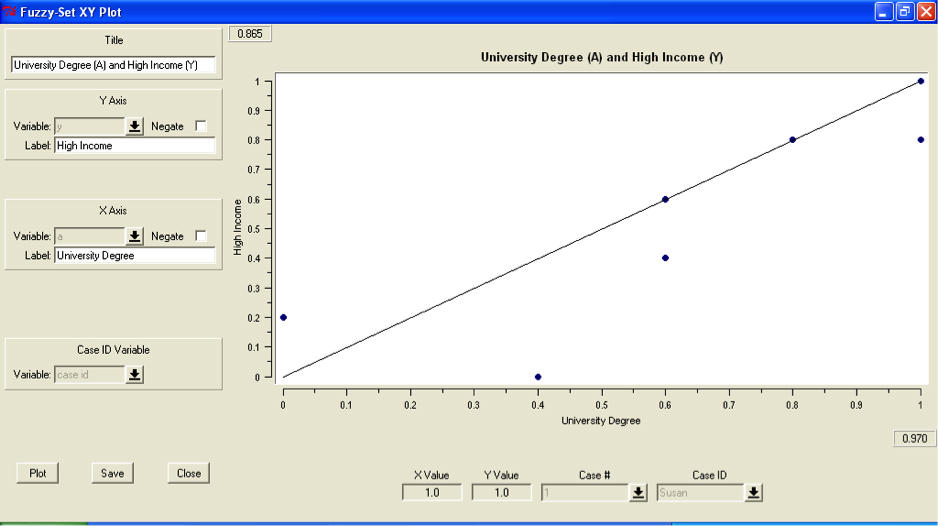
Figure 5: The XY plot window. Please click here for an increased version of Figure 5.
In order to obtain an XY plot, first, you have to specify the causal condition and outcome you are interested in. Click the [↓] button in the [Y Axis] field to select an outcome, and the [↓] button in the [X Axis] field to select a causal condition. To use the negation of either or both sets, check the [negate] box right next to the [↓] buttons. Click the [Plot] button to have the XY plot displayed in the window.21)
Each dot in the plot represents at least one case. Check if more than one case fall onto a given point by clicking on the [↓] button next to the [Case #] field. If more than one case falls onto a point, a list will drop down. The numbers in the lower right and the upper left corner of the graph indicate consistency and coverage. If the upper left number is close to 1.0, this indicates sufficiency; in that case, the lower right corner number displays the coverage. Conversely, a number close to 1.0 in the lower right corner indicates a necessary condition; in that case, the upper left number indicates the coverage. In the example in Figure 5, the visual inspection (almost all cases fall below the main diagonal) as well as the numbers (.97 in the lower right corner) indicate that you are looking at a necessary condition.
You can add a number of further specifications such as a plot title (upper left corner of the window). A very useful option is to specify a case ID variable, which allows you to identify cases within the plot (you need to include a case ID variable in your data set to use this function). The function lets you identify specific cases, e.g., those that deviate from an otherwise consistently necessary or sufficient set relation. To specify a case ID variable, click on the [↓] button in the [Case ID] field. Fs/QCA will let you select any string variable you included in the data set. After plotting the graph, you can see the case IDs of any point by clicking on it in the graph. The case ID will show in the [Case ID] field beneath the plot. Check if more than one case fall onto a given point by clicking on the [↓] button in the field. If more than one case falls onto a point, a list will drop down.
To save XY plots, click on [Save]. The only format available is PostScript files (*.ps). On Macintosh computers, you can view and print this format with the preinstalled Preview software. On PC, you need additional software; a number of freeware options are available.
Through its XY plot function, fs/QCA provides a useful way to visualize your outcomes. Before you can visualize single recipes or your overall solution, you have to compute new variables with the "Compute Variable" function. Click [Variables/Compute] to access the compute console shown in Figure 6. In the [Target Variable] field, you type in the desired name of the new variable, e.g., "RecipeMain."
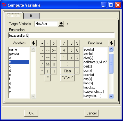
Figure 6: The "Compute Variable" window
To compute a specific recipe, you type in [fuzzyand(condition1, condition2, ...)] in the [Expression] field, with condition1, condition2, etc. representing the causal conditions included in the recipe (a, b in Figure 6). Negations are written as [~condition] within the parentheses. To visualize factorized solutions (see below), create each partial solution in a first step as described above, then combine the new variables via the [fuzzyor] command. In the same way you can visualize combined recipes or the overall solution; create a new condition for each recipe in a first step and connect the new condition via [fuzzyor] in a second step.22)
The computed conditions can be plotted against the outcome using the XY plot function. The consistency score in the upper left corner provides the numerical indicator for the degree to which the recipe, the factorized recipes, or the solution as a whole is consistent with sufficiency for the outcome. The number in the lower right corner indicates the coverage score.
3. Analysis of necessity
One way to analyze the necessity of causal conditions for an outcome is the XY plot tool (see above). Another option that is more time efficient is the necessary conditions tool that can be used by clicking on [Analyze/Necessary Conditions]. A window will open that lets you select the outcome and the causal conditions you want to analyze.
To add single conditions, use the dropdown menu below [Add Condition] to select the condition, then press the [arrow]. The condition will be added to the list. You can add as many conditions as you like. You can add a union of conditions (logical "OR") by selecting a first condition as described above, then using the dropdown menu below [+] to add a further condition.23) When you picked all the conditions you wish to analyze, click [run]. The outcome will be sent to the main QCA window, providing you with the condition names, as well as the consistency and coverage values.
4. Truth table analysis
4.1 Setting up the analysis
To conduct a truth table analysis, click on [Analyze/Fuzzy Sets/Truth Table Algorithm]. A window will open that lets you specify your model, i.e., the outcome set and the conditions you want to include in the analysis. To choose your outcome, select a set and click [Set] or [Set Negated]. To pick the causal conditions you want to include, select them from the list and click [Add].
At the beginning of your research process, it is advisable to include all conditions you deem relevant for the outcome (though not exceeding ten conditions). Later, you should reduce this number by dropping irrelevant conditions and/or conflating conditions that are theoretically and empirically related, since including too many conditions makes the TTA less reliable (MARX, 2006).
If the data set you use includes a case ID variable, you have the option to check the [show solution cases in output] box. Pick the case ID variable from the dropdown menu, and the output will indicate which causal recipe covers which cases.24) This option is very useful because a crucial step in conducting a QCA analysis is reflecting on how well the causal recipes suggested by your TTA work to make sense of the cases they cover.
4.2 Editing the truth table: Frequency and consistency cutoffs
Once you specified your model, click [Run]. A window will open that contains the truth table (see Figure 7). Apart from listing all possible combinations of conditions, the table provides some information on these combinations. The [number] column shows how many empirical instances a configuration has, telling you if it is common, rare, or does not occur at all. This information provides a first insight into causal patterns and matters for your frequency cutoff (see below). The [raw consistency] column tells you how consistently a configuration is a subset of the outcome (that is, satisfies the set relation of sufficiency). This score determines whether to regard a configuration of conditions to consistently contribute to an outcome. The column for the outcome set (the Y column in the table in Figure 7) is left blank since it has to be coded based on the consistency scores and your consistency cutoff.
First, you have to select a frequency cutoff, which determines how many cases a truth table row has to be populated with in order to be included in the analysis. The default setting is one case to populate a truth table row in order for it to be included.25) The configurations of conditions below the threshold will be treated as logical remainders. Second, you will have to choose a consistency cutoff, which determines the threshold at which a combination of conditions is coded as contributing to the outcome. The default setting is .8. While there is no standard threshold, the deterministic notion behind necessity and sufficiency suggests that one should place the consistency cutoff rather higher, say at 0.9 (BRAUMOELLER & GOERTZ, 2000, p.848; SCHNEIDER & WAGEMANN, 2010, p.406).
Sometimes you can find gaps in the consistency scores of configurations. For instance, two configurations have consistency scores close to 1, one has a consistency score of just over .9, and two more configurations have a score of just under .8. In such a case, an option would be to 1. take this distribution of consistency scores into account when choosing the consistency cutoff, and 2. run separate analyses with different cutoffs and compare the recipes suggested by the respective TTAs. If results do not change, this indicates robust findings (SKAANING, 2011).
In some cases, editing the truth table suffices for the program to find the complex, parsimonious, and intermediate solutions to the truth table. In other cases, you need to choose prime implicants and decide on simplifying assumptions first. These steps are explained in the following two sections in the order with which the software proceeds with the analysis; i.e., it will first ask you to choose a prime implicant if necessary, and afterwards ask you for specifications of simplifying assumptions.
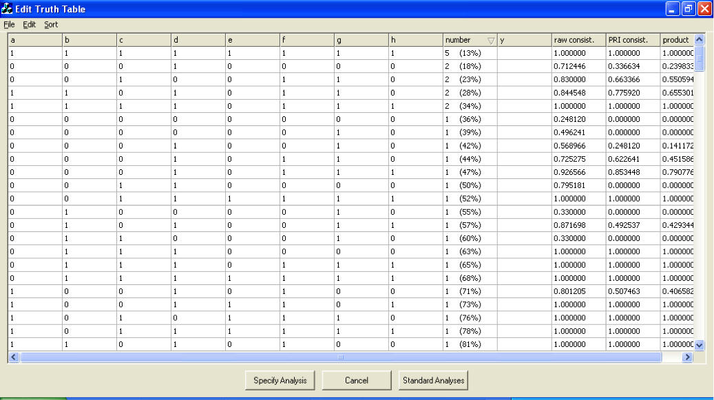
Figure 7: Exemplary truth table (fs/QCA, hypothetical data). Please click here for an increased version of Figure 7.
The most convenient way to choose these settings is to select [Edit/Delete and Code ...] in the truth table window, enter the desired cutoffs, and click [Ok]. The rows not passing the frequency threshold will be treated as a logical remainder and are deleted from the truth table; the rows with consistency scores below your threshold will be coded 0 on the outcome, while those with scores above the threshold will be coded 1. You can also edit the truth table manually, using the [Sort] and [Edit] functions. However, this makes only sense if you wish to edit specific aspects of the truth table instead of just applying a general cutoff for consistency and frequency.
To save the truth table, click [File/Save as CSV File]. Saving the truth table both in its unedited and edited form is important because you should present them as part of your findings from your QCA analysis.
The edited truth table is now ready for minimization. Click [Standard Analysis], which will start the next step of the analysis.
4.3 Selecting prime implicants
At some point in the minimization process, terms cannot be reduced any further. These essential terms are called "prime implicants." For instance, if ABC and AB~C have been reduced to AB, and AB cannot be reduced further through Boolean operations, AB is a prime implicant.
A solution to the minimization of a truth table is only complete if the prime implicants identified cover all primitive expressions. Software packages do this work for you, but sometimes the minimization process results in more prime implicants than are actually needed to cover all primitive expressions. This means that one or more prime implicants are logically redundant. In such cases, the user has to employ substantive and theoretical knowledge to decide which prime implicants to use (SCHNEIDER & WAGEMANN, 2007, pp.69-72).
As with all the choices you make while conducting a TTA, the decision between different prime implicants should be based on theoretical and substantive knowledge. The decision always affects the shape of the parsimonious solution. The intermediate solution might not be affected by this decision at all, but there can be slight or more substantive changes to the intermediate solution, which makes it important to reflect on prime implicants and the choices made. To make decisions explicit and transparent, note which prime implicants were chosen, justify decision when presenting the outcome of a TTA, and check if and in how far the choice affected the intermediate solution. To do so, run the analysis with the different prime implicant options and compare the results in terms of how similar or different they are.
If you need to choose one or more prime implicants, the Prime Implicant Chart window will pop up (see Figure 8).
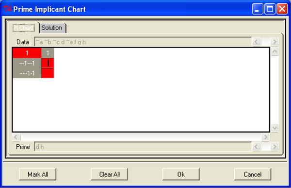
Figure 8: Prime Implicant Chart
The Prime Implicant Chart contains two tabs, [PI Chart] and [Solution]. For the present purpose, only the former is relevant. The first column to the left contains the different prime implicants you may select; each row represents one prime implicant. All further columns in the table represent different truth table rows that are covered by more than one prime implicant. If you click on one of the cells of a given column, the [Data] field above the table will display the corresponding truth table row. By clicking on one of the cells of a row, the [Prime] field below the table will display the respective prime implicant. The number in the top left corner of the table indicates the overall number of prime implicants you need to select in order to cover all truth table rows (in the above case, 1). The red cells in a column indicate which prime implicants could cover that truth table row.
To select a prime implicant, click on the corresponding cell in the first row from the left. The respective cell in the first column will change from grey to white. The number in the upper left corner will decrease by one. When at least one prime implicant is selected for each truth table row, the cell in the upper left corner will show a zero and turn green. You may now proceed with the TTA by clicking [Ok]. To change your selection, you may either right-click on a prime implicant cell you chose, or click the [Clear All] button, and then select again.
4.4 Specifying simplifying assumptions
In a last step before the TTA results show in the main window, you might be asked to specify simplifying assumptions, which determines how logical remainders are treated in the minimization process. Remember that it is of essential importance to invest time in thinking about simplifying assumptions and refrain from using them if you are not sure about how a condition is related to the outcome (BRADY, 2008, pp.220, 236ff.; for a set of criteria for good counterfactuals, see EMMENEGGER, 2010; GRIFFIN, 1993, pp.1101f.).
A separate window opens entitled "Intermediate Solution" (see Figure 9), and you are asked to decide under which circumstances a condition may contribute to the outcome.
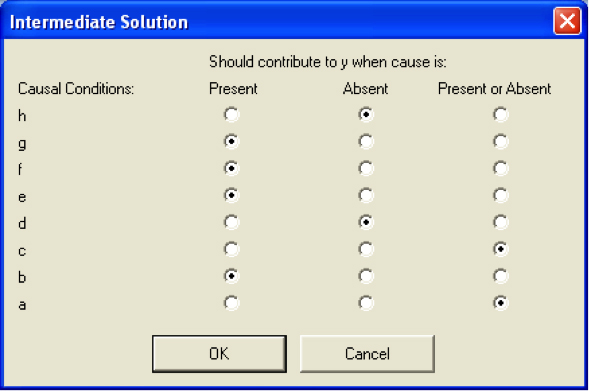
Figure 9: The Intermediate Solution window
For each condition, you have three options for specification. If you are certain that a given condition can only contribute to an outcome if it is present, select [Present]. If you are certain that only the absence of a condition matters for producing the outcome, select [Absent]. Counterfactuals will be used only when the use can be justified based in the respective simplifying assumption. If you are in doubt about whether the presence or absence of a condition contributes to an outcome, or if you are positive that a condition works differently in different environments, select [Present or Absent]. In this case, fs/QCA will not use counterfactuals for minimization that would require any directional expectation for that condition.
4.5 Editing, saving and exporting the output
If you wish to edit the output, e.g., add comments, it is possible to type directly in the output window. To save your output you use [File/Save as/Output] and select a format (e.g., .txt). To export output from fs/QCA, you can just mark it in the main fs/QCA window and copy and paste it into any word-processing software. However, it is crucial to use the right font. Use "Courier New" and adjust the font size so that the tables are represented well in the new file.
4.6 The subset/superset analysis
If you are interested in checking the consistency and coverage score of a specific combination of conditions, you can use the Subset/Superset tool provided by fs/QCA. To conduct a Subset/Superset Analysis, click [Analyze/Subset-Superset Analysis]. A window will pop up that lets you select the causal conditions and the outcome set that you wish to include. Select your causal conditions and click [Add] or [Add Negated], and select your outcome and click [Set] or [Set Negated]. When you specified your model, click [Run]. The output of the analysis will first show up in a separate window. You can edit it by clicking [Edit] and choosing [Delete current row], [Delete current row to last row], or [Delete first row to current row]. Also, you can sort the output by terms, consistency scores, or coverage scores: click on a field in the column you would like to sort by, then click [Sort/Ascending or /Descending]. If you want to revert all changes, click [File/Reset Data]. After editing, you can send the output to the main window by clicking [Send to Output], or you can save it as a .csv file by clicking [File/Save as CSV File].
Appendix 2: List of References for Further Consultation
Immersing oneself in the underlying notions and application of QCA takes time, and it often helps to read different presentations of the same issues in order reach a higher level of confidence in handling concepts, applications, and possible problems of QCA. This appendix collects (non-conclusively) references sorted thematically. It refers the reader to the relevant passages in the main handbooks as well as more specific publications.
|
Theme |
Sources |
|
Handbooks |
Schneider & Wagemann, 2007 (in German) Ragin, 2008 Carmani, 2009 Rihoux & Ragin, 2009 Schneider & Wagemann, 2012 |
|
User's guides |
Ragin, Strand & Rubinson, 2008 Kent, 2008 Schneider, Wagemann & Quaranta, 2012 |
|
Glossaries |
Rihoux & Ragin, 2009, Appendix Schneider & Wagemann, 2012, pp.322-335 |
|
On fuzzy sets |
Zadeh, 1965 Klir & Yuan, 1995 Schneider & Wagemann, 2007, pp.176-179 Ragin, 2008, pp.29-33 Ragin, 2009, pp.89-93 Schneider & Wagemann, 2012, pp.24-31 |
|
On set operations |
Ragin, 2008, pp.34-37 Ragin, 2009, pp.94-98 Schneider & Wagemann, 2012, pp.42-55 |
|
On set calibration |
Schneider & Wagemann, 2007, pp.173-176, 180-183 Ragin, 2008, Chs. 4 and 5 Ragin, 2009, pp.93f. Schneider & Wagemann, 2012, pp.32-41, 232-250 |
|
On necessity and sufficiency |
Braumoeller & Goertz, 2000 Goertz, 2006b Goertz & Levy, 2007 Schneider & Wagemann, 2007, pp.31-43, 197-202 Ragin, 2008, pp.17-23 Pennings, 2009, pp.350-357 Schneider & Wagemann, 2012, pp.56-90 |
|
On consistency and coverage |
Ragin, 2006 Schneider & Wagemann, 2007, pp.86-101, 202-219 Ragin, 2008, Ch. 3 Ragin, 2009, pp.107-109 Schneider & Wagemann, 2012, pp.119-150 |
|
On fuzzy sets and truth tables |
Schneider & Wagemann, 2007, pp.43-73, 188-195, 220-228 Ragin, 2008, Ch. 7 Ragin, 2009, pp.103, 109 Schneider & Wagemann, 2012, pp.178-185, 190-195 |
|
On minimization |
Ragin et al., 2008, pp.37ff. Schneider & Wagemann, 2007, pp.63-73 Schneider & Wagemann, 2012, pp.160-77, 186-189 |
|
On prime implicants |
Schneider & Wagemann, 2007, pp.69-73 Schneider & Wagemann, 2012, pp.109-111 |
|
On limited diversity, simplifying assumptions and counterfactuals |
Schneider & Wagemann, 2007, pp.101-116, 195-197 Ragin, 2008, Chs. 8 and 9 Emmenegger, 2010 Schneider & Wagemann, 2012, pp.151-159, 197-219 |
|
QCA vs. regression analysis |
Ragin, 2004 Katz, Vom Hau & Mahoney, 2005 Clark, Gilligan & Golder, 2006 Schneider & Wagemann, 2007, pp.77-82 Ragin, 2008, Chs. 10 and 11 Grofman & Schneider, 2009 Vis, 2012 |
|
Critiques and discussions |
Seawright, 2005a, 2005b Schneider & Wagemann, 2007, pp.271-273 De Meur et al., 2009, pp.147-165 Pennings, 2009, pp.357-360 |
|
Robustness of results |
Marx, 2006 Skaaning, 2011 Schneider & Wagemann, 2012, pp.284-295 |
|
Standards of good practice |
Schneider & Wagemann, 2007, pp.266-271 Rihoux & Ragin, 2009 Schneider & Wagemann, 2010 Schneider & Wagemann, 2012, pp.275-283 |
|
Resource |
Content |
|
Announcements: events, training, books, newsletter Resources: working paper series, bibliography, overview over software options, useful links |
|
|
Videolectures |
Michael Berthold, 2005 (focus on computer science) |
|
|
Discussions, Q&A, announcements of training opportunities and workshops |
|
|
Schneider, Wagemann & Quaranta, 2012 |
1) I focus on the fuzzy set variant of QCA instead of a crisp set QCA in this article because crisp set QCA is a special case both in terms of practical use and conceptual foundations (SCHNEIDER & WAGEMANN, 2012, p.3). Crisp set QCA operates exclusively with dichotomous conditions (i.e., set values are either 0 or 1), whereas fuzzy set QCA allows values of conditions from 0 to 1. <back>
2) Some authors employ QCA more as an alternative to standard regression analysis (e.g., see GLAESSER, 2008, among others). Such a use of QCA follows a different logic than the one originally intended by RAGIN (e.g., 2008). The present article focuses on the original application of the method. <back>
3) In contrast to the points of full membership and full non-membership, the crossover point should only be a qualitative anchor. For theoretical, practical, and technical reasons, assigning membership scores of 0.5 should be avoided (RAGIN, 2008, p.30; SCHNEIDER & WAGEMANN, 2012, pp.28, 100f.). <back>
4) All examples of data and theoretical arguments used in this article are purely for illustrative purpose and are not meant to contribute to any substantial discussion of the respective research fields. <back>
5) There are few descriptions so far of how this procedure works in practice with qualitative, textual data (for an exception, see SPEER & BASURTO, 2012). When working with numerical instead of textual data sources, it is important not to transform scales "mechanically" into fuzzy sets using some rationale like the median without reflecting on whether this makes theoretical sense (RAGIN, 2008, pp.72f., 2009, p.92; SCHNEIDER & WAGEMANN, 2010, p.403; THIEM, 2010, p.10). Generally speaking, such statistical criteria should only be used when lacking other, more substantial criteria (RIHOUX, 2009a, p.373). <back>
6) For a detailed explanation of the correspondence of logical and set relations, see RAGIN (2008, chapters 2 and 3). <back>
7) The notion of INUS causes was introduced by MACKIE (1965), who described it as "an Insufficient but Necessary part of a condition which is itself Unnecessary but Sufficient for the result" (p.246; my emphases). <back>
8) With A, B, and C, the above truth table has 23=8 rows; i.e., eight different possible configurations of conditions that can represent the cases. By adding a further condition to the truth table, the number of rows would increase to 24 = 16. <back>
9) For a detailed description of how fuzzy sets are represented in truth tables, see, among others, RAGIN (2008, pp.126-133, 2009, pp.99-106) or SCHNEIDER and WAGEMANN (2012, pp.96-104). <back>
10) In the fs/QCA software, the default algorithm used for minimization is Quine-McCluskey (SCHNEIDER & WAGEMANN, 2007, pp.63-73). <back>
11) QCA is not unique in relying on counterfactuals. In fact, they are omnipresent when scholars engage in causal inference, since one can never observe the presence and absence of a given factor within the same case (BRADY, 2008, pp.249-253; GEORGE & BENNETT, 2005, p.230; KING et al., 1994, p.79; MORGAN & WINSHIP, 2007). <back>
12) How the use of counterfactuals is implemented in fs/QCA is discussed in Appendix 1. <back>
13) Some software packages, such as the fuzzy package for Stata (LONGEST & VAISEY, 2008), do not provide this intermediate solution. <back>
14) For a technical step-by-step description of how to use the different tools, see Appendix 1. <back>
15) However, one should be aware that readers not familiar with QCA might mistake XY plots representing set relations for scatterplots showing correlations. Hence, proper explanation is warranted in order to prevent this confusion and point out the relevant features of the plot (SCHNEIDER & GROFMAN, 2006, p.39). <back>
16) Inconsistencies in degree mean that membership in the condition and outcome contradict necessity or sufficiency, but the membership scores lie on the same side of the crossover point (for necessity: A = 0.67, Y = 1; for sufficiency: A = 1, Y = 0.67); an inconsistency in kind means that a case lies on different sides of the crossover point for the condition and the outcome (for necessity: A = 0.33, Y = 1; for sufficiency: A = 1, Y = 0.33). <back>
17) In the course of conducting the TTA with software packages such as fs/QCA, the researcher needs to make a number of specifications and decide at certain points how to go about the analysis, e.g., concerning simplifying assumptions. A step-by-step description of the technical aspect of conducting a TTA using fs/QCA is provided in Appendix 1. <back>
18) In this section I focus on how to incorporate QCA results in within-case analyses. For a discussion of how such qualitative analyses can be conducted see, e.g., BLATTER (2012), GEORGE and BENNETT (2005, pp.205ff.), and GERRING (2007, pp.172ff.). <back>
19) Some scholars suggest that one should not analyze the roles of single conditions in QCA, apart from looking for possible necessary conditions for the outcome (e.g., SCHNEIDER & WAGEMANN, 2010, p.411). I disagree with this stance, following other authors in arguing that it is possible and feasible to analyze the role of single conditions as part of a QCA (e.g., VIS, 2012, p.171). The within-case analysis already provides impressions of what conditions are more relevant overall. QCA can buttress or contradict such impressions, e.g., by showing that a given condition is not part of any combination of conditions that explains the outcome. <back>
20) A note on installation: fs/QCA requires certain user rights that might not be available as a default on company computers. If the data file fails to open, you can try to install the program in the "My Documents" folder and also save your data files in that location. If that fails, consult your system administrator. <back>
21) To produce further plots, you do not need to reopen the window; just specify the new conditions as described and click [Plot] again. <back>
22) You have to use several steps because the program has problems with more complex computing terms. <back>
23) Note that unions of conditions should only be tested for their consistency with necessity if there are theoretical and/or empirical reasons to regard them as interchangeable ways of satisfying a more general condition. It is not uncommon to find quite a few united conditions that are necessary for an outcome because in this case necessity is Y ≤ A+B, with logical OR being defined as max (A, B). Thus, the membership value of A+B is always equal or higher than the membership in A and B separately, increasing the chance of Y ≤ A+B. <back>
24) It is best to check the membership in causal recipes of some cases as indicated in the output against the truth table, since the function sometimes produces flawed results. <back>
25) For most medium N applications of QCA this default setting seems reasonable. Scholars who use QCA to analyze large N data sets often set a higher threshold (e.g., COOPER & GLAESSER, 2012; GLAESSER, 2008, p.203). <back>
References
Basurto, Xavier & Speer, Johanna (2012). Structuring the calibration of qualitative data as sets for qualitative comparative analysis (QCA). Field Methods, 24(2), 155-174.
Berthold, Michael (2005). Tutorial: Fuzzy logic. Videolecture, http://videolectures.net/acai05_berthold_fl/ [Accessed: August 22, 2013].
Blatter, Joachim (2012). Ontological and epistemological foundations of causal-process tracing: Configurational thinking and timing. ECPR Joint Sessions, Antwerpen, April 10-14, 2012. http://www.unilu.ch/files/blatter-taking-terminology-and-timing-seriously-ecpr-antwerp.pdf [Accessed: August 1, 2012].
Brady, Henry E. (2008). Causation and explanation in social science. In Janet M. Box-Steffensmeier, Henry E. Brady & David Collier (Eds.), The Oxford handbook of political methodology (pp.217-270). Oxford: Oxford University Press.
Braumoeller, Bear F. & Goertz, Gary (2000). The methodology of necessary conditions. American Journal of Political Science, 44(4), 844-858.
Carmani, Daniele (2009). Introduction to the comparative method with Boolean algebra. Thousand Oaks, CA: Sage.
Clark, William Roberts; Gilligan, Michael J. & Golder, Matt (2006). A simple multivariate test for asymmetric hypotheses. Political Analysis, 14(3), 311-331.
Cooper, Barry & Glaesser, Judith (2012). Qualitative work and the testing and development of theory: Lessons from a study
combining cross-case and within-case analysis via Ragin's QCA. Forum Qualitative Sozialforschung / Forum: Qualitative Social Research, 13(2), Art.4,
http://nbn-resolving.de/urn:nbn:de:0114-fqs120247 [Accessed: April 10, 2012].
De Meur, Gisele; Rihoux, Benoît & Yamasaki, Sakura (2009). Addressing the critiques of QCA. In Benoît Rihoux & Charles C. Ragin (Eds.), Configurational comparative methods: Qualitative comparative analysis (QCA) and related techniques (pp.147-165). Thousand Oaks, CA: Sage.
Emmenegger, Patrick (2010). How good are your counterfactuals? Assessing quantitative macro-comparative welfare state research with qualitative criteria. COMPASSS Working Paper Series, 59, http://www.compasss.org/wpseries/Emmenegger2010b.pdf [Accessed: April 20, 2010].
George, Alexander L. & Bennett, Andrew (2005). Case studies and theory development in the social sciences. Cambridge: MIT Press.
Gerring, John (2007). Case study research: Principles and practices. Cambridge: Cambridge University Press.
Glaesser, Judith (2008). Just how flexible is the German selective secondary school system? A configurational analysis. International Journal of Research & Method in Education, 31(2), 193-209.
Goertz, Gary (2006a). Social science concepts: A user's guide. Princeton: Princeton University Press.
Goertz, Gary (2006b). Assessing the trivialness, relevance, and relative importance of necessary or sufficient conditions in social science. Studies in Comparative International Development (SCID), 41(2), 88-109.
Goertz, Gary & Levy, Jack S. (2007). Causal explanation, necessary conditions, and case studies. In Gary Goertz & Jack S. Levy (Eds.), Explaining war and peace: Case studies and necessary condition counterfactuals (pp.9-45). New York: Routledge.
Goertz, Gary & Mahoney, James (2005). Two-level theories and fuzzy-set analysis. Sociological Methods & Research, 33(4), 497-538.
Griffin, Larry J. (1993). Narrative, event-structure analysis, and causal interpretation in historical sociology. American Journal of Sociology, 98(5), 1094-1133.
Grofman, Bernard & Schneider, Carsten Q. (2009). An introduction to crisp set QCA, with a comparison to binary logistic regression. Political Research Quarterly, 62(4), 662-672.
Katz, Aaron; Vom Hau, Matthias & Mahoney, James (2005). Explaining the great reversal in Spanish America. Fuzzy-set analysis versus regression analysis. Sociological Methods & Research, 33(4), 539-573.
Kent, Ray (2008). Using fsQCA. A brief guide and workshop for fuzzy-set qualitative comparative analysis, http://www.google.de/url?sa=t&rct=j&q=&esrc=s&source=web&cd=1&ved=0CFsQFjAA&url=http%3A%2F%2Fwww.ccsr.ac.uk%2Fpublications%2Fteaching%2F2008-10.pdf&ei=5N_2T76gEdDIsgbFus33BQ&usg=AFQjCNFZ7Ahwm5efuzy8hkgZcV1ApMdPHA [Accessed: July 6, 2012].
King, Gary; Keohane, Robert O. & Verba, Sidney (1994). Designing social inquiry: Scientific inference in qualitative research. Princeton: Princeton University Press.
Klir, George J. & Yuan, Bo (1995). Fuzzy sets and fuzzy logic: Theory and applications. Upper Saddle River, NJ: Prentice Hall.
Lieberson, Stanley & Lynn, Freda B. (2002). Barking up the wrong branch: Scientific alternatives to the current model of sociological science. Annual Review of Sociology, 28, 1-19.
Longest, Kyle C. & Vaisey, Stephen (2008). fuzzy: A program for performing qualitative comparative analyses (QCA) in Stata. The Stata Journal, 8(1), 79-104.
Mackie, John L. (1965). Causes and conditions. American Philosophical Quarterly, 2(4), 245-264.
Mahoney, James (2012). The logic of process tracing tests in the social sciences. Sociological Methods & Research, 41(4), 570-597.
Mahoney, James & Goertz, Gary (2006). A tale of two cultures: Contrasting quantitative and qualitative research. Political Analysis, 14(3), 227-249.
Marx, Axel (2006). Towards more robust model specification in QCA Results from a methodological experiment. COMPASSS Working Paper Series, 43, http:\www.compasss.org\wpseries\Marx2006.pdf [Accessed: July 15, 2013].
Morgan, Stephen L. & Winship, Christopher (2007). Counterfactuals and causal inference: Methods and principles for social research. Cambridge: Cambridge University Press.
Olson, Wendy (2008a). Qualitative comparative analysis. Videolecture, http://www.methods.manchester.ac.uk/methods/qca/ [Accessed: August 22, 2013].
Olson, Wendy (2008b). What is QCA? Videolecture, http://www.methods.manchester.ac.uk/methods/qca/ [Accessed: August 22, 2013].
Pennings, Paul (2009). Fuzzy-sets and QCA—The methodology of the fuzzy-set logic and its application. In Susanne Pickel, Gert Pickel, Hans-Joachim Lauth & Detlef Jahn (Eds.), Methoden der vergleichenden Politik- und Sozialwissenschaft: Neue Entwicklungen und Anwendungen (pp.347-363). Wiesbaden: VS Verlag für Sozialwissenschaften.
Ragin, Charles C. (1987). The comparative method: Moving beyond qualitative and quantitative strategies. Berkeley, CA: University of California Press.
Ragin, Charles C. (2004). Turning the tables: How case-oriented methods challenge variable-oriented methods. In Henry E. Brady & David Collier (Eds.), Rethinking social inquiry: Diverse tools, shared standards (pp.125-141). Berkeley, CA: Berkeley Institute of Governmental Studies Press.
Ragin, Charles C. (2006). Set relations in social research: Evaluating their consistency and coverage. Political Analysis, 14(3), 291-310.
Ragin, Charles C. (2008). Redesigning social inquiry: Fuzzy sets and beyond. Chicago: University of Chicago Press.
Ragin, Charles C. (2009). Qualitative comparative analysis using fuzzy sets (fsQCA). In Benoît Rihoux & Charles C. Ragin (Eds.), Configurational comparative methods: Qualitative comparative analysis (QCA) and related techniques (pp.87-121). Thousand Oaks, CA: Sage.
Ragin, Charles C. & Davey, Sean (2009). Fuzzy-set/Qualitative comparative analysis 2.5. Tucson, AZ: Department of Sociology, University of Arizona, http://www.u.arizona.edu/~cragin/fsQCA/software.shtml [Accessed: July 13, 2013].
Ragin, Charles C. & Sonnett, John (2005). Between complexity and parsimony: Limited diversity, counterfactual cases, and comparative analysis. In Sabine Kropp & Michael Minkenberg (Eds.), Vergleichen in der Politikwissenschaft (pp.180-197). Wiesbaden: VS Verlag für Sozialwissenschaften.
Ragin, Charles C.; Strand, Sarah I. & Rubinson, Claude (2008). User's guide to fuzzy-set/Qualitative comparative analysis, http://www.u.arizona.edu/~cragin/fsQCA/software.shtml [Accessed: July 6, 2012].
Rihoux, Benoît (2009a). Qualitative comparative analysis (QCA) and related techniques: Recent advances and challenges. In Susanne Pickel, Gert Pickel, Hans-Joachim Lauth & Detlef Jahn (Eds.), Methoden der vergleichenden Politik- und Sozialwissenschaft: Neue Entwicklungen und Anwendungen (pp.365-385). Wiesbaden: VS Verlag für Sozialwissenschaften.
Rihoux, Benoît (2009b). Configurational comparative methods: QCA and fuzzy sets. Videolecture, http://videolectures.net/ssmt09_rihoux_qcafs/ [Accessed: August 22, 2013].
Rihoux, Benoît & Ragin, Charles C. (Eds.) (2009). Configurational comparative methods: Qualitative comparative analysis (QCA) and related techniques. Thousand Oaks, CA: Sage.
Rihoux, Benoît; Álamos-Concha, Priscilla; Bol, Damien; Marx, Axel & Rezsöhazy, Ilona (2013). From niche to mainstream method? A comprehensive mapping of QCA applications in journal articles from 1984 to 2011. Political Research Quarterly, 66(1), 175-184.
Schmitter, Philippe (2008). The design of social and political research. In Donatella Della Porta & Michael Keating (Eds.), Approaches and methodologies in the social sciences: A pluralist perspective (pp.263-295). Cambridge: Cambridge University Press.
Schneider, Carsten Q. & Grofman, Bernard (2006). It might look like a regression equation ... but It's not! An intuitive approach to the presentation of QCA and fs/QCA results. COMPASSS Working Paper Series, 39, http://www.compasss.org/wpseries/SchneiderGrofman2006.pdf [Accessed: July 15, 2013].
Schneider, Carsten Q. & Wagemann, Claudius (2007). Qualitative Comparative Analysis (QCA) und Fuzzy Sets: Ein Lehrbuch für Anwender und jene, die es werden wollen. Opladen: Budrich.
Schneider, Carsten Q. & Wagemann, Claudius (2010). Standards of good practice in qualitative comparative analysis (QCA) and fuzzy-sets. Comparative Sociology, 9(3), 397-418.
Schneider, Carsten Q. & Wagemann, Claudius (2012). Set-theoretic methods for the social sciences: A guide to qualitative comparative analysis. Cambridge: Cambridge University Press.
Schneider, Carsten Q.; Wagemann, Claudius & Quaranta, Mario (2012). How to ... Use software for set-theoretic analysis: Online appendix to "set-theoretic methods for the social sciences", http://www.cambridge.org/servlet/file/Howtosoftware.pdf?ITEM_ENT_ID=7093279&ITEM_VERSION=2&COLLSPEC_ENT_ID=842&download=1 [Accessed: November 12, 2012].
Seawright, Jason (2005a). Assumptions, causal inference, and the goals of QCA. Studies in Comparative International Development (SCID), 40(1), 39-42.
Seawright, Jason (2005b). Qualitative comparative analysis vis-à-vis regression. Studies in Comparative International Development (SCID), 40(1), 3-26.
Skaaning, Svend-Erik (2011). Assessing the robustness of crisp-set and fuzzy-set QCA results. Sociological Methods & Research, 40(2), 391-408.
Strauss, Anselm L. & Corbin, Juliet M. (1998). Basics of qualitative research: Grounded theory procedures and techniques. Thousand Oaks: Sage.
Thiem, Alrik (2010). Set-relational fit and the formulation of transformational rules in fsQCA. COMPASSS Working Paper Series, 61, http://www.compasss.org/wpseries/Thiem2010.pdf [Accessed: May 19, 2011].
Thomson, Steph (2012). QCA. Videolecture, http://www.methods.manchester.ac.uk/methods/qca/ [Accessed: August 22, 2013].
Vis, Barbara (2012). The comparative advantages of fsQCA and regression analysis for moderately large-N analyses. Sociological Methods & Research, 41(1), 168-198.
Wagemann, Claudius & Schneider, Carsten Q. (2010). Qualitative comparative analysis (QCA) and fuzzy-sets: Agenda for a research approach and a data analysis technique. Comparative Sociology, 9(3), 376-396.
Zadeh, Lofti A (1965). Fuzzy sets. Information and Control, 8, 338-853.
Author
|
Nicolas LEGEWIE is a doctoral student at the Berlin Graduate School of Social Sciences and Humboldt-University of Berlin. He is writing his dissertation on educational upward mobility among students from low socioeconomic backgrounds. His research interests include social inequality, education, immigration, social networks, as well as research methodology. |
Contact: Nicolas Legewie Berlin Graduate School of Social Sciences E-mail: nicolas.legewie@hu-berlin.de |
Legewie, Nicolas (2013). An Introduction to Applied Data Analysis with Qualitative Comparative Analysis (QCA) [88 paragraphs].
Forum Qualitative Sozialforschung / Forum: Qualitative Social Research, 14(3), Art. 15,
http://nbn-resolving.de/urn:nbn:de:0114-fqs1303154.

Creative Commons Attribution 4.0 International License